library(ggplot2)
library(lme4)
library(emmeans)Mixed model simulation
statistics
simulation
I have started to believe that a good part of understanding the process of a particular statistical model involves being able to set up a simulation of it. Here we do a simulation of data expected from a fish gut microbiota pilot study that I was involved in
Let’s go
While we obtain abundance data on many different microbes at once (a community profile) in such studies, the first step is to understand what we can do with just one. This means this approach is applicable to each microbe separately and does not examine the data at community level.
In this simulation, there are 4 gut locations (mouth, foregut, midgut and hindgut) examined from 10 fish (A to J).
The model is:
\[Y_{abundance} = beta1_{gut.location} + sigma1_{fish} + sigma2_{unexplained}\]
Packages
Building the data set
There are 4 gut locations and 10 fish, thus there are 40 * 10 rows required.
fish_data <-
  expand.grid(
    gut_location = c("mouth", "foregut", "midgut","hindgut"),
    fish_id = LETTERS[1:10]
  ) |>
  tibble::as_tibble()

fish_data
# A tibble: 40 × 2
gut_location fish_id
<fct> <fct>
1 mouth A
2 foregut A
3 midgut A
4 hindgut A
5 mouth B
6 foregut B
7 midgut B
8 hindgut B
9 mouth C
10 foregut C
# ℹ 30 more rowsDefine parameters
Let’s assume these proportion trends and that there are about 200 individuals. This gives us the deterministic part of the model.
gut_location_proportion <-
  c("mouth" = 0.01,
    "foregut" = 0.5,
    "midgut" = 0.35,
    "hindgut" = 0.10
  )

gut_location_means <- 200 * gut_location_proportion

gut_location_means
mouth foregut midgut hindgut
2 100 70 20 Next we define the variability of fish individuals and unexplained variation.
set.seed(1010)

fish_variation <-
  rnorm(10, sd = 15) |>
  round(digits = 0) |>
  setNames(unique(fish_data$fish_id))

fish_variation
A B C D E F G H I J
2 -13 20 6 -4 20 29 -35 -9 -8 residual_variation <-
rnorm(n = nrow(fish_data), sd = 5) |>
round(0)
residual_variation [1] -1 -4 -7 0 4 -4 -4 1 -5 -5 0 4 -5 2 -3 4 -2 -5 -1 -9 -5 10 -1 2 -5
[26] 2 -1 -2 -3 -5 -2 2 0 3 -3 1 2 -3 2 7Simulating the counts
Then we use the above to create observed counts
set.seed(1010)

fish_data_build <-
  fish_data |>
  dplyr::mutate(
    location_count = gut_location_means[gut_location],
    fish_variation = fish_variation[fish_id],
    residual_variation = residual_variation,
    observed_count = location_count + fish_variation + residual_variation,
    observed_count = ifelse(observed_count < 0, 0, observed_count)
  )

fish_data_build
# A tibble: 40 × 6
gut_location fish_id location_count fish_variation residual_variation
<fct> <fct> <dbl> <dbl> <dbl>
1 mouth A 2 2 -1
2 foregut A 100 2 -4
3 midgut A 70 2 -7
4 hindgut A 20 2 0
5 mouth B 2 -13 4
6 foregut B 100 -13 -4
7 midgut B 70 -13 -4
8 hindgut B 20 -13 1
9 mouth C 2 20 -5
10 foregut C 100 20 -5
# ℹ 30 more rows
# ℹ 1 more variable: observed_count <dbl>And lastly, clean up the data
fish_data_final <-
  fish_data_build |>
  dplyr::select(gut_location, fish_id, observed_count)

fish_data_final
# A tibble: 40 × 3
gut_location fish_id observed_count
<fct> <fct> <dbl>
1 mouth A 3
2 foregut A 98
3 midgut A 65
4 hindgut A 22
5 mouth B 0
6 foregut B 83
7 midgut B 53
8 hindgut B 8
9 mouth C 17
10 foregut C 115
# ℹ 30 more rowsData exploration
Counts by fish individuals
fish_data_final |>
  ggplot(aes(x = gut_location, y = observed_count, group = fish_id)) +
  geom_line()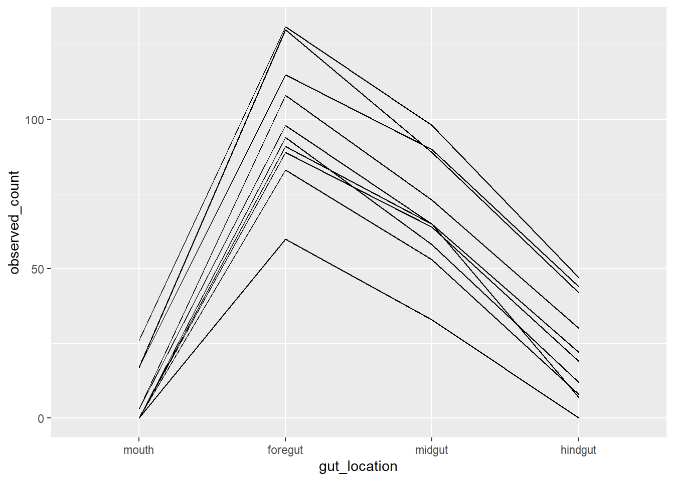
In another way
fish_data_final |>
  ggplot(aes(x = gut_location, y = observed_count, group = fish_id)) +
  geom_line() +
  geom_point() +
  facet_wrap(vars(fish_id), nrow = 2)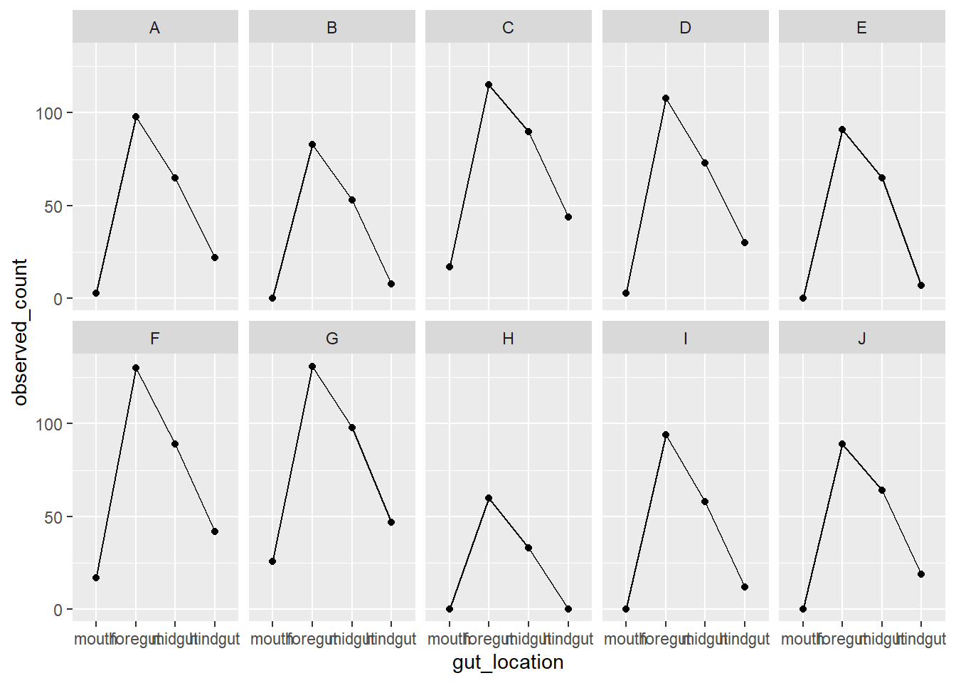
Hand calculating parameters
fish_data_final |>
  dplyr::group_by(gut_location) |>
  dplyr::summarise(
    mean_count = mean(observed_count)
  )
# A tibble: 4 × 2
gut_location mean_count
<fct> <dbl>
1 mouth 6.6
2 foregut 99.9
3 midgut 68.8
4 hindgut 23.1fish_data_final |>
dplyr::group_by(fish_id) |>
dplyr::summarise(
mean_count = mean(observed_count)
) |>
dplyr::ungroup() |>
dplyr::summarise(
sd_count = sd(mean_count)
)# A tibble: 1 × 1
sd_count
<dbl>
1 16.5Modelling
We fit the model like so
fit1 <- lmer(observed_count ~ gut_location + (1|fish_id), data = fish_data_final)

plot(fit1, pch = 19)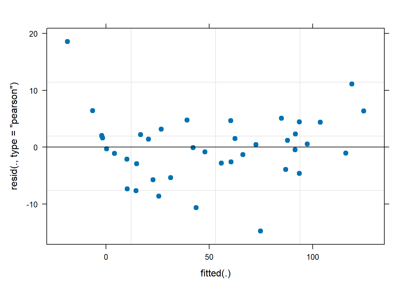
And obtain a model summary
fit1_summary <- summary(fit1)
fit1_summary
Linear mixed model fit by REML ['lmerMod']
Formula: observed_count ~ gut_location + (1 | fish_id)
Data: fish_data_final
REML criterion at convergence: 279.4
Scaled residuals:
Min 1Q Median 3Q Max
-2.10601 -0.40453 0.02645 0.36144 2.65347
Random effects:
Groups Name Variance Std.Dev.
fish_id (Intercept) 259.93 16.122
Residual 48.95 6.997
Number of obs: 40, groups: fish_id, 10
Fixed effects:
Estimate Std. Error t value
(Intercept) 6.600 5.558 1.188
gut_locationforegut 93.300 3.129 29.818
gut_locationmidgut 62.200 3.129 19.879
gut_locationhindgut 16.500 3.129 5.273
Correlation of Fixed Effects:
(Intr) gt_lctnf gt_lctnm
gt_lctnfrgt -0.281
gt_lctnmdgt -0.281 0.500
gt_lctnhndg -0.281 0.500 0.500 And we obtain the values we used for the data simulation
fit1_summary$coefficients Estimate Std. Error t value
(Intercept) 6.6 5.557727 1.187536
gut_locationforegut 93.3 3.128957 29.818245
gut_locationmidgut 62.2 3.128957 19.878830
gut_locationhindgut 16.5 3.128957 5.273323fit1_summary$varcor Groups Name Std.Dev.
fish_id (Intercept) 16.1224
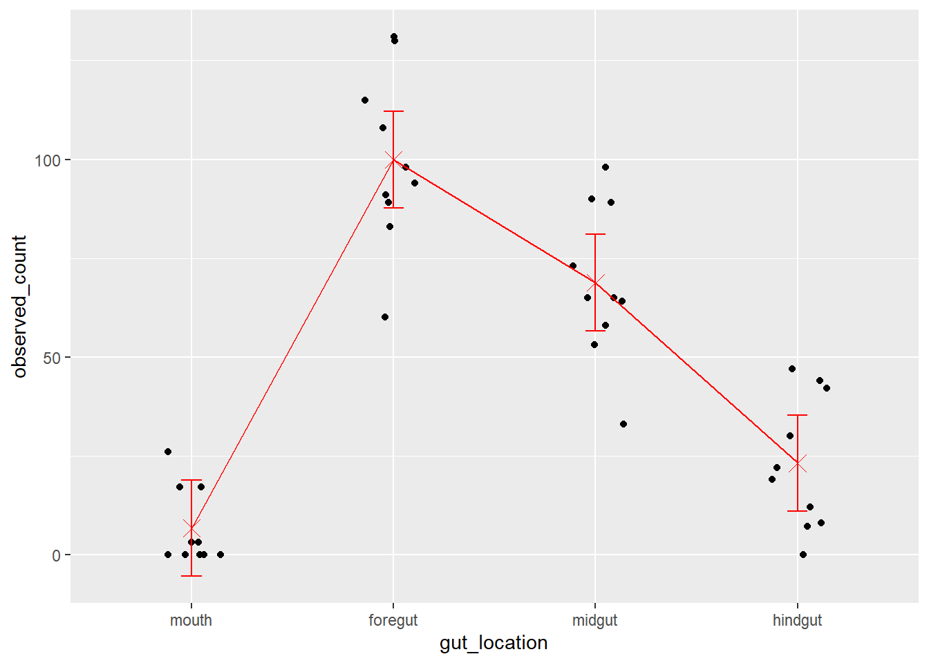
Residual 6.9966 Lastly, a final plot …
fit1_means <-
  emmeans::emmeans(fit1, specs = 'gut_location') |>
  as.data.frame()
Cannot use mode = "kenward-roger" because *pbkrtest* package is not installedfish_data_final |>
ggplot(aes(x = gut_location, y = observed_count)) +
geom_jitter(height = 0, width = 0.15) +
geom_point(data = fit1_means,
mapping = aes(y = emmean),
color = 'red', size = 4, shape = 'cross') +
geom_line(data = fit1_means,
mapping = aes(y = emmean, group = 1),
color = 'red') +
geom_errorbar(data = fit1_means,
mapping = aes(y = NULL, ymax = upper.CL, ymin = lower.CL),
color = 'red',
width = 0.1)